StatPCA — Principal Component Analysis Workbench

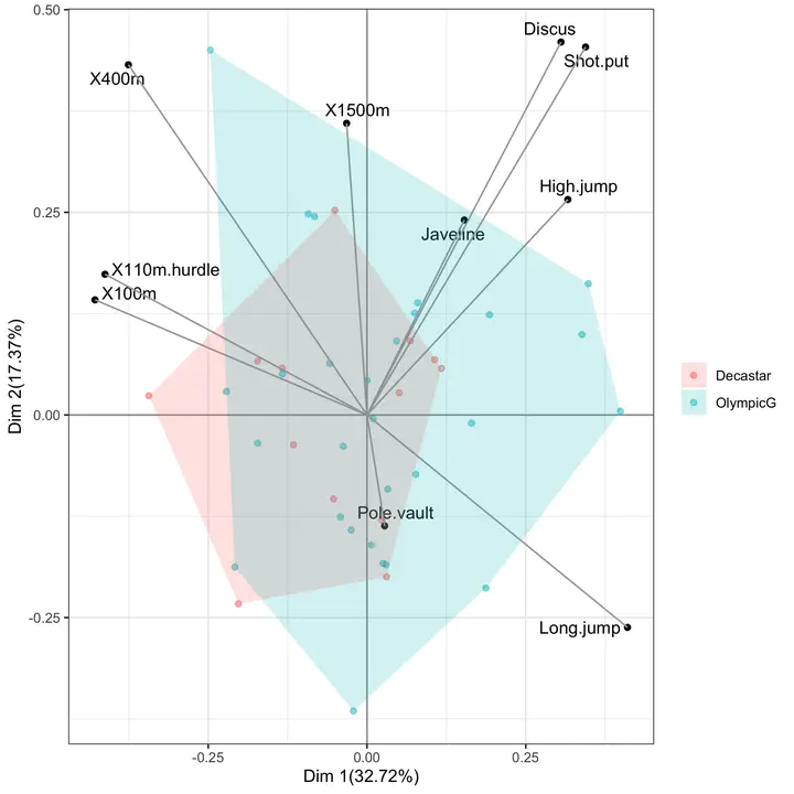
A browser-only teaching workbench for the most-used dimension-reduction technique in applied multivariate statistics: Principal Component Analysis. StatPCA completes the family of teaching tools developed for undergraduate and graduate statistics at Qatar University, alongside StatTables, StatTests, StatRegress, StatCI, StatPower, and StatCorr.

Why a PCA workbench?

Principal Component Analysis is often presented as a one-line recipe — “decompose the correlation matrix and keep the first few eigenvectors” — and the geometric, algebraic, and inferential layers of the method are collapsed into a single black-box call. StatPCA keeps the layers separate and visible: the data panel makes the centering and scaling step explicit, the eigen-decomposition panel reports eigenvalues and eigenvectors of the chosen matrix, the variance panel reports the scree plot and the cumulative proportion of variance explained, and the projection panel renders the score plot, the loading plot, and the biplot on coordinated axes.

What the app does

Input. Paste a CSV with $p \geq 2$ numeric variables, load one of the bundled teaching datasets (e.g., the classical decathlon, USArrests, or iris), or generate synthetic correlated data with a user-specified covariance structure. Categorical or grouping variables are kept aside and used only to colour the score plot.

Pre-processing options. Mean-centering is applied by default; the user toggles between PCA on the correlation matrix (each variable scaled to unit variance) and PCA on the covariance matrix (variables left on their original scale). Missing values are handled by listwise deletion or by mean-imputation, with both options reported next to the result.

Quantities reported. For every fit the app returns:

• the eigenvalues $\lambda_{1} \geq \lambda_{2} \geq \cdots \geq \lambda_{p} \geq 0$ of the chosen matrix, with their proportion $\lambda_{k}/\sum_{j}\lambda_{j}$ and cumulative proportion;
• the loadings matrix $\mathbf{V} = (v_{jk})$ with columns equal to the eigenvectors of the chosen matrix; loadings are reported on the unit-norm scale and on the correlation-with-component scale $v_{jk}\sqrt{\lambda_{k}}$, so that the user can read off the linear association between each original variable and each component;
• the scores $z_{ik} = \sum_{j} v_{jk},(x_{ij}-\bar x_{j})/s_{j}$ of each observation on each component;
• the communalities and the squared cosines $\cos^{2}_{ik}$, which quantify how well each observation is represented in the chosen low-dimensional subspace.

Visual output. The app renders three coordinated plots:

1. the scree plot with the broken-stick and Kaiser ($\lambda > 1$) reference lines superimposed, so that the choice of the number of retained components is grounded in an explicit rule rather than visual judgement alone;
2. the score plot of observations on $(\text{PC}{k}, \text{PC}{\ell})$, with optional colouring by a grouping variable and confidence ellipses per group;
3. the biplot, which overlays the loading vectors on the score plot using the standard scaling so that the cosine of the angle between two arrows approximates the correlation between the corresponding variables.

Pedagogical use

StatPCA is designed for the lecture in which PCA is introduced and for the practical that follows it. Three exercises map naturally to the app:

1. Standardisation matters. Run PCA on the covariance matrix of a dataset whose variables are on incompatible scales (e.g., heights in cm and weights in kg), then re-run on the correlation matrix and watch the dominant component swap. Discuss when each choice is appropriate.
2. How many components? Compare the Kaiser rule, the broken-stick rule, and the elbow-on-the-scree-plot rule on the same data. Show that they need not agree, and connect the disagreement to the eigenvalue spectrum.
3. Interpreting the axes. Use the loadings (on the correlation-with-component scale) to label the principal axes in substantive terms; use the squared cosines to flag observations that the two-dimensional summary represents poorly.

Technical notes

The app is a single-page client-side application built with React + Vite: all computation runs in the student’s browser, with no server round-trip and no data leaving the device. The eigen-decomposition is performed by a numerically stable QR-based routine on the symmetric correlation/covariance matrix; for the score plot the app uses the singular value decomposition of the centered (and optionally scaled) data matrix, which avoids forming and squaring the cross-product matrix when the number of variables is large. The static bundle is deployed on Netlify; like its siblings it works offline after first load and has no external run-time dependencies.